August, 2020 | Music Informatics Group

Multi-Task Learning for Instrument Activation Aware Music Source Separation

by Yun-Ning Hung

Motivation

Music source separation performance has been improved dramatically in recent years due to the rise of deep learning, especially in the fully-supervised learning setting. However, one of the main problems of the current music source separation systems is the lack of large-scale datasets for training. Most of the open-source datasets either have limited size, or the number of included instruments and music genres is limited.

Moreover, many existing systems focus exclusively on the problem of source separation itself and ignore the utilization of other possibly related MIR tasks which could lead to additional quality gain.

In this research work, we leverage two open-source large-scale multi-track datasets, MedleyDB and Mixing Secrets, in addition to the standard MUSDB to evaluate on a large variety of separable instruments. We also propose a multitask learning structure to explore the combination of instrument activity detection and music source separation. The goal is that by training these two tasks in an end-to-end manner, the estimated instrument labels can be used during inference as a weight for each time frame. We refer to our method as instrument aware source separation (IASS).

Model structure

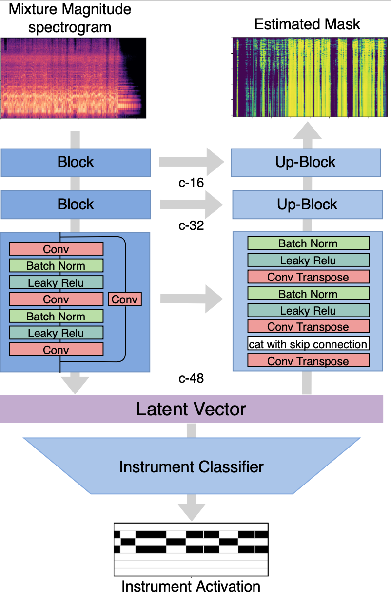
Our proposed model is a U-net based structure with residual blocks instead of CNNs at each layer. The reason for choosing the U-net structure is that it has been found useful in image decomposition, a task with general similarities to source separation. The residual block allows the information from the current layer to be fed into a layer 2 hops away and deepens the structure. A classifier is attached to the latent vector to predict the instrument activity. Mean Square Error (MSE) loss is used for source separation while Binary Cross-Entropy (BCE) loss is used for instrument activity prediction.

Instrument weight

Figure 2: Using instrument activation as a weight to filter the estimated mask, which will be used to multiply with the mixture of the magnitude spectrogram.

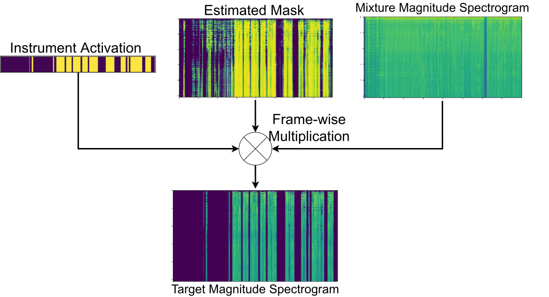
We use instrument activation as a weight to multiply with the estimated mask along the time dimension. By doing so, the instrument labels are able to suppress the frames not containing any target instrument. The instrument activation is first binarized by using a threshold. A median filter is then applied to smooth the estimated activation.

Experiments & Results

We compare our model with baseline Open-Unmix model. Both models use mixture phase without any post-processing. We train and evaluate both models on two datasets, MUSDB-HQ dataset and the combination of Mixing Secrets and MedleyDB.

Figure 3: BSS metrics for Open-Unmix and IASS on the MUSDB-HQ dataset.

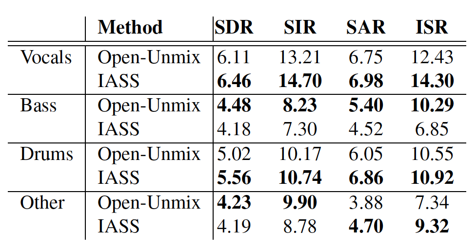
The result shows that when training and evaluating on the MUSDB-HQ dataset, our model outperforms the Open-Unmix model on ‘Vocals’ and ‘Drums’, performs equally on ‘Other’, and slightly worse on ‘Bass’. This might be because ‘Bass’ is likely to appear throughout the songs; as a result, the improvement of using the instrument activation weight is limited.

Figure 4: SDR score for Open-Unmix, IASS, an ideal binary mask and input-SDR.

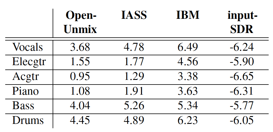
Figure 4 summarizes the results for the combination of the MedleyDB and Mixing Secrets datasets. The Ideal Binary Mask (IBM) represents the best-case scenario. The worst-case scenario is represented by the results for input-SDR, which is the SDR score when using the unprocessed mixture as the input. We can observe that our model also outperforms Open-Unmix on all the instruments. Moreover, both models have higher scores on ‘Drums,’ ‘Bass,’ and ‘Vocals’ than on ‘Electrical Guitar’, ‘Piano’, and ‘Acoustic Guitar’. This might be attributed to the fact that ‘Guitar’, ‘Piano’, and ‘Acoustic Guitar’ have fewer training samples. Another possible reason is that the more complicated spectral structure of polyphonic instruments such as ‘Guitar’ and ‘Piano’ make the separation task more challenging.

Conclusion

This work presents a novel U-net based model that incorporates instrument activity detection with source separation. We also utilize a larger dataset to evaluate various instruments. The result shows our model achieves equal or better separation quality than the baseline model. Future extension of this work includes:

Increasing the amount of data by using a synthesized dataset,
Incorporating other tasks, such as multi-pitch estimation, into our current model, and
Exploring post-processing methods such as Wiener filter, to improve our system’s quality.

Resources

The code for reproducing experiments is available on our Github repository.
Please see the full paper (to appear in ISMIR ’20) for more details on the dataset and our experiment.

AR-VAE: Attribute-based Regularization of VAE Latent Spaces

by Ashis Pati

In the context of deep generative models, improving controllability by enabling selective manipulation of data attributes has been an active area of research. Latent representation-based models such as Variational Auto-Encoders (VAEs) have shown promise in this direction as they are able to encode certain hidden attributes of the data.

In this research work, we propose a supervised training method which uses a novel regularization loss to create structured latent spaces where specific continuous-valued attributes are forced to be encoded along specific dimensions of the latent space. For instance, if the attributes represents ‘thickness’ of a digit, and the regularized dimensions correspond to the first dimension of the latent space, then sampling latent vectors with increasing values of the first dimension should result in the same digit with increased thickness. This overall idea is shown in Figure 1 below. The resulting Attribute-Regularized VAE (AR-VAE) can then be used to manipulate these attributes by simple traversals along the regularized dimension.

Figure 1: Overall schematic of the AR-VAE model.

AR-VAE has several advantages over previous methods. Unlike Fader Networks it is designed to work with continuous-valued attributes, and unlike GLSR-VAE, it is agnostic to the way attributes are computed or obtained.

Method

In order to create a structured latent space where an attribute $a$ is encoded along a dimension $r$, we add a novel attribute regularization loss to the standard VAE-objective. This loss is designed such that as we traverse along $r$, the attribute value $a$ of the generated data increases. To formulate the loss function, we consider a mini-batch of $m$ examples, and follow a three-step process:

1. Compute an attribute distance matrix $D_a$
2. Compute a regularized dimension distance matrix $D_r$
3. Compute the mean absolute error between signs of $D_a$ and $D_r$

In practice, we compute the hyperbolic tangent of $D_r$ so as to ensure differentiability of the loss function with respect to the latent vectors. Multiple regularization terms can be used to encode multiple attributes simultaneously. For a more detailed mathematical description of the loss function, check out the full paper.

Experimental Results

We evaluated AR-VAE using different datasets from the image and music domains. Here, we present some of the results of manipulating different attributes. For detailed results on other experiments such as latent space disentanglement, reconstruction fidelity, content preservation, and hyperparameter tuning, check out the full paper.

Manipulation of Image Attributes

Manipulating attributes of 2-d shapes. Each row in the figure below represents a unique shape (from top to bottom): square, heart, ellipse. Each column corresponds to traversal along a regularized dimension which encodes a specific attribute (from left to right): Shape, Scale, Orientation, x-position, y-position.

Manipulating attributes of MNIST digits. Each row in the figure below represents a unique digit from 0 to 9. Each column corresponds to traversal along a regularized dimension which encodes a specific attribute (from left to right): Area, Length, Thickness, Slant, Width, Height.

Manipulation of Musical Attributes

Manipulating attributes of monophonic measures of music. In the figure below, measures on each staff line are generated by traversal along a regularized dimension which encodes a specific musical attribute (shown on the extreme left).

Piano-roll version of the figure above is shown below. Plots on the right of each piano-roll show the progression of attribute values.

Conclusion

Overall, AR-VAE creates meaningful attribute-based interpolations while preserving the content of the original data. In the context of music, it can be used to build interactive tools or plugins to aid composers and music creators. For instance, composers would be able to manipulate different attributes (such as rhythmic complexity) of the composed music to try different ideas and meet specific compositional requirements. This would allow fast iteration and would be especially useful for novices and hobbyists. Since the method is agnostic to how the attributes are computed, it can potentially be useful to manipulate high-level musical attributes such as tension and emotion. This will be particularly useful for music generation in the context of video games where the background music can be suitably changed to match the emotional context of the game and the actions of the players.

Resources

dMelodies: A Music Dataset for Disentanglement Learning

by Ashis Pati

Motivation

In the field of machine learning, it is often required to learn low-dimensional representations which capture important aspects of given high-dimensional data. Learning compact and disentangled representations (see Figure 1) from given data, where important factors of variation are clearly separated, is considered especially useful for generative modeling.

Figure 1: Disentangled representation learning.

However, most of the current/previous studies on disentanglement have relied on datasets from the image/computer vision domain (such as the dSprites dataset).

We propose dMelodies, a standardized dataset for conducting disentanglement studies on symbolic music data which will allow:

researchers working on disentanglement algorithms evaluate their method on diverse domains.
systematic and comparable evaluation of methods meant specifically for music disentanglement.

dMelodies Dataset

To enable objective evaluation of disentanglement algorithms, one needs to either know the ground-truth values of the underlying factors of variation for each data point, or be able to synthesize the data points based on the values of these factors.

Design Principles

The following design principles were used to create the dataset:

It should have a simple construction with homogeneous data points and intuitive factors of variation.
The factors of variation should be independent, i.e., changing any one factor should not cause changes to other factors.
There should be a clear one-to-one mapping between the latent factors and the individual data points.
The factors of variation should be diverse and span different types such as discrete, ordinal, categorical and binary.
The generated dataset should be large enough to train deep neural networks.

Dataset Construction

Based on the design principles mentioned above, dMelodies is artificially generated dataset of simple 2-bar monophonic melodies generated using 9 independent latent factors of variation where each data point represents a unique melody based on the following constraints:

Each melody will correspond to a unique scale (major, harmonic minor, blues, etc.).
Each melody plays the arpeggios using the standard I-IV-V-I cadence chord pattern.
Bar 1 plays the first 2 chords (6 notes), Bar 2 plays the second 2 chords (6 notes).
Each played note is an 8th note.

A typical example is shown below in Figure 2.

Factors of Variation

The following factors of variation are considered:

1. Tonic (Root): 12 options from C to B
2. Octave: 3 options from C4 through C6
3. Mode/Scale: 3 options (Major, Minor, Blues)
4. Rhythm Bar 1: 28 options based on where the 6 note onsets are located in the first bar.
5. Rhythm Bar 2: 28 options based on where the 6 note onsets are located in the second bar.
6. Arpeggiation Direction Chord 1: 2 options (up/down) based on how the arpeggio is played
7. Arpeggiation Direction Chord 2: 2 options (up/down)
8. Arpeggiation Direction Chord 3: 2 options (up/down)
9. Arpeggiation Direction Chord 4: 2 options (up/down)

Consequently, the total number of data-points are 1,354,752.

Benchmarking Experiments

We conducted benchmarking experiments using 3 popular unsupervised algorithms (beta-VAE, Factor-VAE, and Annealed-VAE) on the dMelodies dataset and compared the result with those obtained using the dSprites dataset. Overall, we found that while disentanglement performance across different domains is comparable (see Figure 3), maintaining good reconstruction accuracy (see Figure 4) was particularly hard for dMelodies.

Figure 3: Disentanglement performance (higher is better) in terms of Mutual Information Gap (MIG) of different methods on the dMelodies and dSprites datasets.

Figure 4: Reconstruction accuracies (higher is better) of the different methods on the dMelodies and dSprites datasets. For reconstruction, the median accuracy for 2 methods fails to cross 50% which makes them unusable in a generative modeling setting.

Thus, methods which work well for image-based datasets do not extend directly to the music domain. This showcases the need for further research on domain-invariant algorithms for disentanglement learning. We hope this dataset is a step forward in that direction.

Resources

The dataset is available on our Github repository. The code for reproducing our benchmarking experiments is available here. Please see the full paper (to appear in ISMIR ’20) for a more in-depth discussion on the dataset design process and additional results from the benchmarking experiments.